Statistics Primer

Once tracing is complete and the data collected. The next step in analyzing it is to leverage some descriptive statistics to get a feeling for the data. TracerBench will handle this for you and provided within the various TracerBench Reports.

Population & Sample

Population and Sample are part of the foundation of statistical hypothesis testing.
A population is a collection of data which you want to make an assumption on. For example in a swimming pool of water this represents all of the water in the pool. Since testing every drop of water is not realistically possible. A subset of the population (subset of the pool water) is tested to analyze and make an assumption, which is called a sample.
To represent the population well, a sample should be randomly collected and adequately large. If the sample is random and large enough, you can use the information collected from the sample to make an assumption about the larger population. Then leverage a hypothesis test to estimate the percentage of the sample to the population.

Probability Sampling

Sampling involves choosing a method of sampling (how are we going to sample). In the example of the swimming pool, are we going to only sample the pool water from the shallow end? deep end? both ends? The method we decide on will influence the data we result with.
The two major categories in sampling are probability and non-probability sampling. For a given population (swimming pool), each element (drop of water) of that population has a chance of being "picked" as part of the sample (cup of water). In other words, no single element of the population has a zero chance of being picked. The odd/chances/probability of picking any element is known or can be calculated. This is possible if we know the total number in the entire population and are able to determine the odds of picking any one element. Probability sampling involves randomly picking elements from a population which is why no element has a zero chance of being picked to be part of a sample.

Null hypothesis (H0)

The null hypothesis is a statement about a population. A hypothesis test uses sample data to determine whether to reject the null hypothesis. The null hypothesis states that a population parameter (such as the mean, the standard deviation, etc.) is equal to a hypothesized value. The null hypothesis is often an initial claim that is based on a previous analysis or insights.

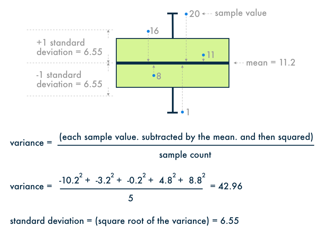
Standard Deviation & Variance

The standard deviation is the most common measure of how spread out the data are from the mean (dispersion). The greater the standard deviation, the greater the spread in the data.
The variance measures how much the data is scattered about their mean. The variance is equal to the standard deviation squared.

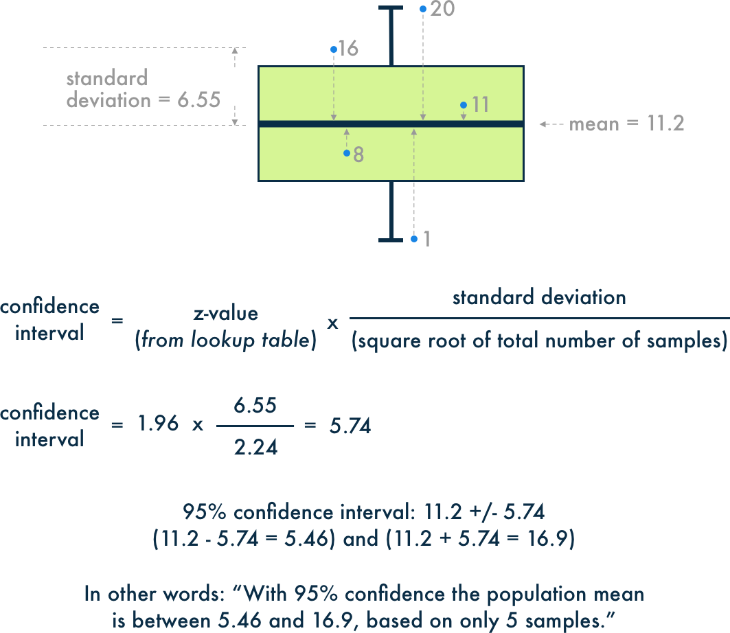
Confidence Interval

A confidence interval is a range of values, derived from sample statistics, that is likely to contain the value of an unknown population parameter. Since they are random it's unlikely that two samples from a population will yield identical confidence intervals. However, if the sampling is repeated many times, a certain percentage of the confidence intervals would contain the unknown population parameter. For example in a 95% confidence interval, 5% would contain the unknown population parameter.
Confidence intervals are commonly more useful than hypothesis tests because they provide a way to assess practical significance in addition to statistical significance. They help you determine what parameter value is, instead of what it is not.

Power

The power of a hypothesis test is the probability that the test correctly rejects the null hypothesis. The power of a hypothesis test is affected by the sample size, difference, variance and the significance level of the test.
If a test has low power, you might fail to detect an effect and mistakenly conclude that none exists. If a test has a power that is too high very small effects/changes might seem to be significant.

Wilcoxon rank sum with continuity correction

Wilcoxon rank sum essentially calculates the difference between each set of pairs in the test and analyzes the differences in the pairs. Continuity correction essentially is as simple as adding or subtracting 0.5 to the x-value of a distribution with a lookup table to determine when to add or subtract 0.5.

Statistical Significance

Statistical significance itself doesn't imply that your results have practical consequence. If you use a test with very high power, you might conclude that a small difference from the hypothesized value is statistically significant. However, that small difference might be meaningless to your situation. Your technical insight should be leveraged to determine whether the difference is practically significant. With a large enough sample, you can likely reject the null hypothesis even though the difference is of no practical importance.
(sources: https://cbmm.mit.edu, https://www.wyzant.com, https://support.minitab.com)